2013-02-02

Some theory

I created this blog because I replicate quite a few finance papers with R and I thought that some of you might profit from some of my work. Note, however, that I consider myself a mediocre R user! I'm still one of those guys that uses Stackoverflow mainly for asking questions, not for answering them...so I'm sure that my approach isn't always the most efficient one and if you have any comments on how to improve my code, let me know!

OK, let's start with Goyal/Welch (2008): A Comprehensive Look at The Empirical Performance of Equity Premium Prediction, Review of Financial Studies. You find the paper and the data on Amit Goyal's webpage. That's what I love about finance research nowadays...data is available from the authors, so all you have to do is to download it and you can play around with it yourself.

What's this paper all about? Well, there is a huge literature on "return predictability": you take a predictor, such as the dividend-price ratio or the consumption-wealth ratio, and you try to forecast future excess returns with it. Note that the very idea of return predictability is a paradigm change from the early days, when the random-walk hypothesis implied stock returns that are close to unpredictable. Nowadays, economists argue that stock returns have to be predictable. Why? One big reason is that we have a changing price-dividend ratio over time. If future dividend growth and expected returns were i.i.d., the price-dividend ratio would have to be constant. Thus a changing price-dividend ratio means that one of the two must be forecastable; and research indicates that returns should be the more relevant part here. To read more about that topic, check out chapter 20 in Cochrane (2005, Asset Pricing) or his presidential address to the AFA.

As already mentioned, there are now tons of papers that deal with return predictability. Goyal/Welch point out that the literature has become so big, with many different predictors, methods, and data sets, that it is quite tough to absorb. Hence, the goal of their article (taken from Goyal/Welch, 2008, p. 1456)

is to comprehensively re-examine the empirical evidence as of early 2006, evaluating each variable using the same methods (mostly, but not only, in linear models), time-periods, and estimation frequencies. The evidence suggests that most models are unstable or even spurious. Most models are no longer signiﬁcant even insample (IS), and the few models that still are usually fail simple regression diagnostics. Most models have performed poorly for over 30 years IS. For many models, any earlier apparent statistical signiﬁcance was often based exclusively on years up to and especially on the years of the Oil Shock of 1973–1975. Most models have poor out-of-sample (OOS) performance, but not in a way that merely suggests lower power than IS tests. They predict poorly late in the sample, not early in the sample. (For many variables, we have difﬁculty ﬁnding robust statistical signiﬁcance even when they are examined only during their most favorable contiguous OOS sub-period.) Finally, the OOS performance is not only a useful model diagnostic for the IS regressions but also interesting in itself for an investor who had sought to use these models for market-timing. Our evidence suggests that the models would not have helped such an investor.

Therefore, although it is possible to search for, to occasionally stumble upon, and then to defend some seemingly statistically signiﬁcant models, we interpret our results to suggest that a healthy skepticism is appropriate when it comes to predicting the equity premium, at least as of early 2006. The models do not seem robust.

Replication

In my opinion, the most interesting part about this paper is that they don't bother to look at any regression coefficients. So the results are very different from what you usually see in such papers. Basically, they just look at the mean squared errors (MSE) (from Wikipedia: In statistics, the mean squared error (MSE) of an estimator is one of many ways to quantify the difference between values implied by an estimator and the true values of the quantity being estimated. MSE is a risk function, corresponding to the expected value of the squared error loss or quadratic loss. MSE measures the average of the squares of the errors.) and transform the MSE to several useful statistics:

$$ \begin{aligned} R^2 &= 1 - \frac{MSE_A}{MSE_N} \\ \Delta RMSE &= \sqrt{MSE_N} - \sqrt{MSE_A}\\ \end{aligned} $$ where $h$ is the degree of overlap ($h=1$ for no overlap). Note that $MSE_N=E[e_N^2]$ and $MSE_A=E[e_A^2]$, where $e_N$ denote the vector of rolling OOS errors from the historical mean model and $e_A$ denote the vector of rolling OOS from the OLS model. Now, this is very important so let's think about this for a while: many scholars within the return predictability literature argue that a bunch of variables forecast equity premiums. Goyal/Welch (2008) now use the same test with the same time period for all those variables and compare it to the simplest of all forecasting techniques: the simple historic average. Note, however, that these statistics only apply to the OOS tests. For the IS tests, $R^2$ is just the R squared you know from a linear regression, and $\overline{R}^2$ is the adjusted one.

Data

The data is taken from Amit Goyal's webpage. There is an updated version from 2010. However, I'm using the original data from 2005, so I can easily control the correctness of my computations. Also, I repeat some definitions of the appendix here:

Stock Variance (svar): Stock Variance is computed as sum of squared daily returns on S&P 500. Daily returns for 1871 to 1926 are obtained from Bill Schwert while daily returns from 1926 to 2005 are obtained from CRSP
Cross-Sectional Premium (csp): The cross-sectional beta premium measures the relative valuations of high- and low-beta stocks. We obtained this variable directly from Sam Thompson. This variable is available from May 1937 to December 2002
NetEquity Expansion (ntis) is the ratio of twelve-month moving sums of net issues by NYSE listed stocks divided by the total market capitalization of NYSE stocks
Long Term Yield (lty): Long-term government bond yields for the period 1919 to 1925 is the U.S. Yield On Long-Term United States Bonds series from NBER’s Macrohistory database. Yields from 1926 to 2005 are from Ibbotson’s Stocks, Bonds, Bills and Inﬂation Yearbook
Long Term Rate of Return (ltr): Long-term government bond returns for the period 1926 to 2005 are from Ibbotson’s Stocks, Bonds, Bills and Inﬂation Yearbook
The Term Spread (tms) is the diﬀerence between the long term yield on government bonds and the T-bill
Inﬂation (inﬂ): Inﬂation is the Consumer Price Index (All Urban Consumers) for the period 1919 to 2005 from the Bureau of Labor Statistics. Because inﬂation information is released only in the following month, in our monthly regressions, we inserted one month of waiting before use Inﬂation (inﬂ): Inﬂation is the Consumer Price Index (All Urban Consumers) for the period 1919 to 2005 from the Bureau of Labor Statistics. Because inﬂation information is released only in the following month, in our monthly regressions, we inserted one month of waiting before use.

The monthly, quarterly, and annual data is saved in one Excel file. To read that into R, I have split this excel file into three CSV-files. Now it's easy to read them in. Also, I convert them into data.tables because I prefer to work with them instead of data.frames. Finally, I use the package lubridate to convert the column Datum into a date. You have to name this column yourself in the CSV-file!

library(data.table)
library(ggplot2)
library(lubridate)
library(dyn)
library(reshape2)
monthly <- read.csv2("/home/christophj/Dropbox/FinanceIssues/ReturnPredictability/Data/monthly_2005.csv", 
                     na.strings="NaN", stringsAsFactors=FALSE)
annual  <- read.csv2("/home/christophj/Dropbox/FinanceIssues/ReturnPredictability/Data/annual_2005.csv", 
                     na.strings="NaN", stringsAsFactors=FALSE)
monthly <- as.data.table(monthly)
annual  <- as.data.table(annual)
monthly <- monthly[, Datum := ymd(Datum)]

First of all, we have to compute the dividend price ratio (d/p) and the dividend yield (d/y). They are defined as the difference between the log of dividends and the log of prices and as the difference between the log of dividends and the log of lagged prices. Also, we have to compute the equity premium as the difference of the S&P returns and the risk-free rate. A few things to notice here:

It took me a while to get the same summary statistics as in Goyal/Welch (2008). A few problems here: Goyal always provides updated data on his website. The problem with this data is that it not only adds new data points, but it also changes the historical data. For instance, the dividends were slightly adjusted. Hence, to get the same results as in Goyal/Welch (2008), you have to use the original data set.
Also, you have to figure out if everything is defined in simple or log returns. They explain it in table 1 of their 2003 Management Science paper ("Predicting the Equity Premium with Dividend Ratios") more clearly: "(The expected return) $Rm(t)$ is the log of the total return on the value-weighted stock market from year $t-1$ to $t$. (The equity premium) $EQP(t)$ subtracts the equivalent log return on a three-month treasury bill. $DP(t)$ is the dividend-price ratio, i.e., the log of aggregate dividends $D(t)$ divided by the aggregate stock market value $P(t)$. $DY(t)$, the dividend-yield ratio, divides by $P(t-1)$ instead... All variables are in percentages."
The rest is try and error. Doing so, you will find out that the risk-free rate is provided in simple, not log returns, so you have to do that yourself.

So let's calculate the relevant variables, i.e. the log equity premium (rp_div), dividend-price ratio (dp), and the dividend yield (dy), and plot them over time:

annual <- annual[, IndexDiv := Index + D12]
annual <- annual[, dp := log(D12) - log(Index)]
annual <- annual[, ep := log(E12) - log(Index)]
vec_dy <- c(NA, annual[2:nrow(annual), log(D12)] - annual[1:(nrow(annual)-1), log(Index)])
annual <- annual[, dy := vec_dy]
annual <- annual[, logret   :=c(NA,diff(log(Index)))]
vec_logretdiv <- c(NA, annual[2:nrow(annual), log(IndexDiv)] - annual[1:(nrow(annual)-1), log(Index)])
vec_logretdiv <- c(NA, log(annual[2:nrow(annual), IndexDiv]/annual[1:(nrow(annual)-1), Index]))
annual <- annual[, logretdiv:=vec_logretdiv]
annual <- annual[, logRfree := log(Rfree + 1)]
annual <- annual[, rp_div   := logretdiv - logRfree]
#Put it in time series (is needed in function get_statistics)
ts_annual <- ts(annual, start=annual[1, Datum], end=annual[nrow(annual), Datum])
plot(ts_annual[, c("rp_div", "dp", "dy")])

This yields exactly the same equity premia as in Goyal/Welch (2008, p. 1457), more precisely a mean (standard deviation) of the log equity risk premium of 4.84% (17.79%) for the complete sample from 1872 to 2005; of 6.04% (19.17%) from 1927 to 2005; and of 6.04% (15.70%) from 1965 to 2005.

Also, a look at the figure is interesting, which replicates figure 1 from Goyal/Welch (2003). They write "... that there is some nonstationarity in the dividend ratios. The dividend ratios are almost random walks, while the equity premia are almost i.i.d. Not surprisingly, the augmented Dickey and Fuller (1979) test indicates that over the entire sample period, we cannot reject that the dividend ratios contain a unit-root (see Stambaugh 1999 and Yan 1999)."

Define function

Next, we want to replicate the plots in Goyal/Welch (2008), i.e. we plot the cumulative squared predictions errors of the NULL (simple average mean) minus the cumulative squared prediction error of the ALTERNATIVE, where the ALTERNATIVE is a model that relies on a predictive variable to forecast the equity premium. We also give some summary statistics.

This is all done in one function. This function takes a data.frame (note that a data.table is just a data.frame) (ts_df), the independent variable (indep), the dependent variable (dep), the degree of overlap (h), the start year (start) , the end year (end), and the OOS period (OOS_period), which basically decides how many periods are used to compute the out-of-sample statistics.

A few comments on the function (I hope the rest is self-explanatory, otherwise leave a comment):

The function window expects a time-series. This is why we called the function ts further above. The function window is quite convenient in subsetting a data set based on the date.
The package dyn is used to easily run regressions with a lagged variable.
In general, the lines in which I call functions like eval, parse, etc. might be quite confusing. This looks quite complicated, but allows me to select the variables in ts_df dynamically. I'm confused about how this actually works myself, so for me it's mostly try and error. Hadley Wickham's webpage is quite helpful though.

get_statistics <- function(ts_df, indep, dep, h=1, start=1872, end=2005, est_periods_OOS = 20) {

  #### IS ANALYSIS

  #1. Historical mean model
  avg   <- mean(window(ts_df, start, end)[, dep], na.rm=TRUE)
  IS_error_N <- (window(ts_df, start, end)[, dep] - avg)

  #2. OLS model
  reg <- dyn$lm(eval(parse(text=dep)) ~ lag(eval(parse(text=indep)), -1), data=window(ts_df, start, end))
  IS_error_A <- reg$residuals
  ### 

  ####OOS ANALYSIS
  OOS_error_N <- numeric(end - start - est_periods_OOS)
  OOS_error_A <- numeric(end - start - est_periods_OOS)
  #Only use information that is available up to the time at which the forecast is made
  j <- 0
  for (i in (start + est_periods_OOS):(end-1)) {
    j <- j + 1
    #Get the actual ERP that you want to predict
    actual_ERP <- as.numeric(window(ts_df, i+1, i+1)[, dep])

    #1. Historical mean model
    OOS_error_N[j] <- actual_ERP - mean(window(ts_df, start, i)[, dep], na.rm=TRUE)

    #2. OLS model
    reg_OOS <- dyn$lm(eval(parse(text=dep)) ~ lag(eval(parse(text=indep)), -1), 
                      data=window(ts_df, start, i))
    #Compute_error
    df <- data.frame(x=as.numeric(window(ts_df, i, i)[, indep]))
    names(df) <- indep
    pred_ERP   <- predict.lm(reg_OOS, newdata=df)
    OOS_error_A[j] <-  pred_ERP - actual_ERP

  }


  #Compute statistics 
  MSE_N <- mean(OOS_error_N^2)
  MSE_A <- mean(OOS_error_A^2)
  T <- length(!is.na(ts_df[, dep]))
  OOS_R2  <- 1 - MSE_A/MSE_N
  #Is the -1 enough (maybe -2 needed because of lag)?
  OOS_oR2 <- OOS_R2 - (1-OOS_R2)*(reg$df.residual)/(T - 1) 
  dRMSE <- sqrt(MSE_N) - sqrt(MSE_A)
  ##

  #### CREATE PLOT
  IS  <- cumsum(IS_error_N[2:length(IS_error_N)]^2)-cumsum(IS_error_A^2)
  OOS <- cumsum(OOS_error_N^2)-cumsum(OOS_error_A^2)
  df  <- data.frame(x=seq.int(from=start + 1 + est_periods_OOS, to=end), 
                    IS=IS[(1 + est_periods_OOS):length(IS)], 
                    OOS=OOS) #Because you lose one observation due to the lag
  #Shift IS errors vertically, so that the IS line begins 
  # at zero on the date of first OOS prediction. (see Goyal/Welch (2008, p. 1465))
  df$IS <- df$IS - df$IS[1] 
  df  <- melt(df, id.var="x") 
  plotGG <- ggplot(df) + 
    geom_line(aes(x=x, y=value,color=variable)) + 
    geom_rect(data=data.frame(),#Needed by ggplot2, otherwise not transparent
              aes(xmin=1973, xmax=1975,ymin=-0.2,ymax=0.2), 
              fill='red',
              alpha=0.1) + 
    scale_y_continuous('Cumulative SSE Difference', limits=c(-0.2, 0.2)) + 
    scale_x_continuous('Year')
  ##

  return(list(IS_error_N = IS_error_N,
              IS_error_A = reg$residuals,
              OOS_error_N = OOS_error_N,
              OOS_error_A = OOS_error_A,
              IS_R2 = summary(reg)$r.squared, 
              IS_aR2 = summary(reg)$adj.r.squared, 
              OOS_R2  = OOS_R2,
              OOS_oR2 = OOS_oR2,
              dRMSE = dRMSE,
              plotGG = plotGG))

}

Now, we can easily replicate the plots in Goyal/Welch (2008). All we need to do is type two lines of code. Let's start!

In-sample analysis (IS)

Dividend-price ratio

dp_stat <- get_statistics(ts_annual, "dp", "rp_div", start=1872)
dp_stat$plotGG

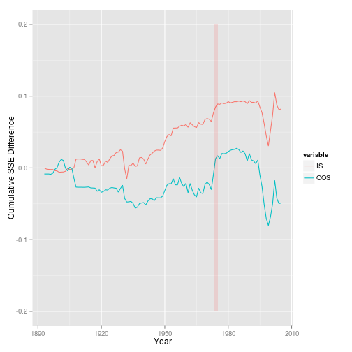
This figure looks exactly like the chart in Figure 1 of Goyal/Welch (2008), but my statistics are very different. Particularly the $\overline{R}^2$, which is 0.48% and 0.49% for them.

Dividend-yield

dy_stat <- get_statistics(ts_annual, "dy", "rp_div", start=1872)
dy_stat$plotGG

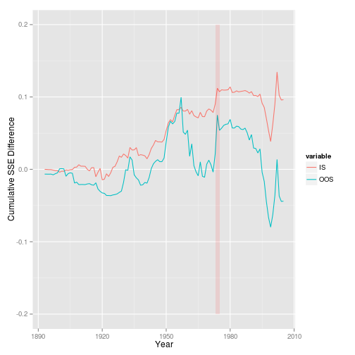
Statistics: $\overline{R}^2$, which is 0.90% and 0.91% for them.

Earnings-price ratio

ep_stat <- get_statistics(ts_annual, "ep", "rp_div", start=1872)
ep_stat$plotGG

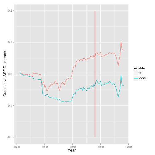
Statistics: $\overline{R}^2$, which is 1.10% and 1.08% for them.

So this post showed you how to reproduce the plots of Goyal/Welch (2008) with R. Note that this post is meant to show you how easily this can be done with R, not to replicate exactly the statistics in their paper. A few things are off (plots are not exactly identical, $\overline{R{IS}}^2$ is not always correct, my $\overline{R{OOS}}^2$ is wrong), but since I get basically the same results as they do, I don't have the motivation right now to figure out where the really small deviations are coming from. Feel free to tell me if you figure it out, though.

Replicating Goyal/Welch (2008)