Replicating Cochrane (2008)
In this post, I want to replicate some results of Cochrane (2008), The Dog That Did Not Bark: A Defense of Return Predictability, Review of Financial Studies, 21 (4). You can find that paper on John Cochrane's website. I wrote some thoughts about return predictability already on my Goyal/Welch replication post, so please check this one out for some more background. Or just read the papers, they explain it better than I could anyway.
Replication of the forecasting regressions in Cochrane's Table 1
Let's first repeat the forecasting regressions Cochrane runs in Table 1 of his paper. He uses data in real terms, i.e. deflated by the CPI, and on an annual basis ranging from 1926 to 2004. I do not have access to CRSP, but fortunately, we find similar data on Robert Shiller's website. His data is saved in an Excel-file and is formatted in such a way that you cannot just read it into R. So you manually have to delete unnecessary rows and save the sheet Data as a .CSV file. Also, here is the naming convention I apply for the relevant columns:
- RealR: Real One_Year Interest Rate (column H as of february 2013). Note that Cochrane uses real return on 3-month Treasury-Bills, but I'm to lazy to find that somewhere else and match it.
- RealP: RealP Stock Price (column P as of february 2013).
- RealD: RealD S&P Dividend (column O as of february 2013).
- Ret_SP: Return on S&P Composite (column P as of february 2013).
- Year: First column with the years.
library(data.table)
#CHANGE TO THE DIRECTORY IN WHICH YOU SAVED THE FILE
strPath <- "/home/christophj/Dropbox/R_Package_Development/vignettes_REM/Data/Robert_Shiller_Data_Formatted.csv"
#strPath <- "C:/Dropbox/R_Package_Development/vignettes_REM/Data/Robert_Shiller_Data_Formatted.csv"
shiller_data <- as.data.table(read.csv(strPath))
strStart <- 1924; strEnd <- 2005
#GET RELEVANT DATA
shiller_data <- shiller_data[, Dgrowth := c(NA, exp(diff(log(RealD))))]
shiller_data <- shiller_data[, DP := RealD/RealP]
vec_Ret_SP <- c(NA, shiller_data[2:nrow(shiller_data), RealP + RealD]/shiller_data[1:(nrow(shiller_data)-1), RealP ])
shiller_data <- shiller_data[, Ret_SP := vec_Ret_SP]
shiller_data <- shiller_data[, Ex_Ret_SP := Ret_SP - RealR]
shiller_data <- shiller_data[Year >= strStart & Year <= strEnd, list(Ret_SP, Ex_Ret_SP, RealR, RealD, Dgrowth, DP)]
summary(shiller_data)
##      Ret_SP        Ex_Ret_SP           RealR           RealD
##  Min.   :0.616   Min.   :-0.5297   Min.   :0.853   Min.   : 6.43
##  1st Qu.:0.948   1st Qu.:-0.0554   1st Qu.:0.993   1st Qu.:10.13
##  Median :1.101   Median : 0.0791   Median :1.018   Median :14.05
##  Mean   :1.091   Mean   : 0.0750   Mean   :1.016   Mean   :13.39
##  3rd Qu.:1.218   3rd Qu.: 0.1928   3rd Qu.:1.036   3rd Qu.:17.22
##  Max.   :1.539   Max.   : 0.5534   Max.   :1.146   Max.   :22.68
##     Dgrowth            DP
##  Min.   :0.647   Min.   :0.0110
##  1st Qu.:0.983   1st Qu.:0.0312
##  Median :1.021   Median :0.0406
##  Mean   :1.022   Mean   :0.0413
##  3rd Qu.:1.062   3rd Qu.:0.0514
##  Max.   :1.499   Max.   :0.0806
With the summary statistics, you can check if you get the same results as I do. Now we have all the ingredients to run the regressions.
Since we have to lag the independent variable by one year, I use the R package dyn, which makes lagging easier. However, we have to convert our data.table to a time-series object first with the ts function.
library(dyn)
library(xtable)
ts_data <- ts(data=shiller_data, start=strStart, end=strEnd)
list_reg <- list(reg_R_DP = dyn$lm(Ret_SP ~ lag(DP, -1), data=ts_data),
                 reg_ER_DP = dyn$lm(Ex_Ret_SP ~ lag(DP, -1), data=ts_data),
                 reg_Dgrowth_DP = dyn$lm(Dgrowth ~ lag(DP, -1), data=ts_data),
                 reg_r_dp = dyn$lm(log(Ret_SP) ~ log(lag(DP, -1)), data=ts_data),
                 reg_dgrowth_dp = dyn$lm(log(Dgrowth) ~ log(lag(DP, -1)), data=ts_data),
                 reg_dp_next_dp = dyn$lm(log(DP) ~ log(lag(DP, -1)), data=ts_data))
tab <- t(as.data.frame(lapply(list_reg[1:5], FUN = function(reg) {
      c(b  = summary(reg)$coef[2,1],
        t  = summary(reg)$coef[2,3],
        R2 = summary(reg)$adj.r.sq * 100,
        sd = sd(reg$fitted) * 100)
      })))
#Covariance matrix from table 2
#cor(cbind(list_reg[[4]]$resid, list_reg[[5]]$resid, list_reg[[6]]$resid))
#apply(cbind(list_reg[[4]]$resid, list_reg[[5]]$resid, list_reg[[6]]$resid), 2, sd)
print(xtable(tab), type="HTML")
| b | t | R2 | sd | |
|---|---|---|---|---|
| reg_R_DP | 3.19 | 2.23 | 4.73 | 4.76 |
| reg_ER_DP | 3.45 | 2.31 | 5.14 | 5.14 |
| reg_Dgrowth_DP | 0.26 | 0.32 | -1.13 | 0.39 |
| reg_r_dp | 0.09 | 1.91 | 3.22 | 3.95 |
| reg_dgrowth_dp | 0.00 | 0.12 | -1.25 | 0.15 |
Technically, it is a nice trick to save objects like the regression results in lists. (Note that if I would have had more regressions to run here, I would have written a small customed function in which the dependent and independent variables can be passed dynamically. However, for five regressions this isn't really necessary). Now you can loop through every object of the list with lapply and apply a function on that object. In the above example, I just return the four elements I'm interested in: regression coefficient, t-value, adjusted $R^2$, and standard deviation of the fitted values of the regression.
As you can see, the regressions work by and large. Both returns and expected returns have a positive and significant regression coefficient, although mine is slightly lower than Cochrane's. This also leads to lower t-values. Also, I get a positive regression coefficient for the dividend growth regression that is close to one. As a side note: This data set probably assumes that dividends are reinvested in the stock market. For instance, Koijen/van Nieuwerburgh (2011) argue that it is better to reinvest dividends at the risk-free rate. Otherwise, what you actually measure are the properties of the stock market, i.e. realized returns, not realized dividends. Since you want to distinguish between the two, you should be careful here. They show results that actually give evidence for dividend growth predictability in the correct direction, i.e. high dividend-price ratios predict low future dividend growth.
To the interpretation: Slope coefficients around 3 in the top two row mean that when "dividend yields rise one percentage point, prices rise another two percentage points on average, rather than declining one percentage point to offset the extra dividends and render returns unpredictable" (Cochrane, 2008, p. 1533).
The basic set up
He goes on and sets up a simple first-order VAR representation that simultaneously models log returns, log dividend yields, and log dividend growth:
Now, let's simulate the VAR and assume that returns are not predictable. We can then test how likely it is in this case that we observe predictability for returns, but not for dividend growth, in the data. To simulate the VAR, we use the parameters as provided in Table 2 of Cochrane (2008), $\phi=0.941$, and $\rho=09638$. However, I write a function so that I can play around with the values later on.
How does the function work? Well, the core idea of the paper is that log dividend growth, log returns, and log price-dividend ratios are related. So we actually only have to choose two variables to simulate to start with and the third one can then be computed with the Campbell/Shiller identity. Cochrane chooses the dividend-growth and the dividend yield because those two have uncorrelated shocks, so they are easy to simulate.
The simulations
simulate_data <- function(nrT = 77, phi=0.941, rho=0.9638, vec_sd = c(0.196, 0.14, 0.153)) {

  #Set up vectors
  shocks_dp <- rnorm(nrT + 1, sd=vec_sd[3])
  shocks_d  <- rnorm(nrT, sd=vec_sd[2])
  vec_dp <- numeric(nrT+1)

  #Draw first observation for dividend yield
  ifelse(phi >= 1, vec_dp[1] <- 0, vec_dp[1] <- rnorm(1, sd=vec_sd[3]^2/(1-phi^2)))

  #Simulate the system forward
  for (i in 2:(nrT+1)) {
    vec_dp[i] <- phi * vec_dp[i-1] + shocks_dp[i]
  }
  vec_d <- (phi*rho - 1) * vec_dp[1:nrT] + shocks_d
  vec_r <- shocks_d - rho * shocks_dp[2:(nrT+1)]

  return(data.frame(dp = vec_dp[2:(nrT+1)],
                    div_growth = vec_d,
                    ret = vec_r))

}
This is the function to simulate the data. The most confusing part of this function is the fact that we need an additional element in the dividend yield vector. Since the dividend yield of the last period determines today's dividend yield and dividend growth, we need a start value for the dividend yield.
Next, we want to run a Monte Carlo simulation in which we draw many samples, run the regressions given above and get some statistics of that. So let's write this function:
run_MCS <- function(nrMCS = 50000, ...) {

  reg_coef <- matrix(nrow=nrMCS, ncol=6)

  for (i in 1:nrMCS) {

    #1. Simulate data
    ts_data <- ts(simulate_data(...))

    #2. Run regressions
    list_reg <- list(dyn$lm(ret ~ lag(dp, -1), data=ts_data),
                     dyn$lm(div_growth ~ lag(dp, -1), data=ts_data),
                     dyn$lm(dp ~ lag(dp, -1), data=ts_data))

    #3. Get regression coefficients and t-values
    reg_coef[i, 1:3] <- unlist(lapply(list_reg,
                                      FUN = function(reg) summary(reg)$coef[2,1]))
    reg_coef[i, 4:6] <- unlist(lapply(list_reg,
                                      FUN = function(reg) summary(reg)$coef[2,3]))

  }

  reg_coef <- as.data.frame(reg_coef)
  reg_n <- c("ret", "div_growth", "dp")
  names(reg_coef) <- c(paste0("Coef_", reg_n), paste0("tValue_", reg_n))
  return(reg_coef)

}
Now we have all the ingredients to replicate Table 3 and Figure 1 in Cochrane (2008). Note that he is silent on how long one run actually is, i.e. what nrT should be in simulate_data. However, since he calibrates the regressions with 77 years of data, I'm gonna assume that this is the time period he is simulating per run.
nrMCS <- 50000; phi <- 0.941; rho <- 0.9638
reg_coef <- run_MCS(nrMCS = nrMCS, phi=phi, rho=rho, nrT = 77 , vec_sd = c(0.196, 0.14, 0.153))
Now, we can check if we get the same results as Cochrane in the first row of his Table 3.
sum(reg_coef$Coef_ret > 0.097)/nrMCS*100
## [1] 26.51
sum(reg_coef$tValue_ret > 1.92)/nrMCS*100
## [1] 9.318
sum(reg_coef$Coef_div_growth > 0.008)/nrMCS*100
## [1] 2.662
sum(reg_coef$Coef_div_growth > 0.18)/nrMCS*100
## [1] 0.006
And we can reproduce the plots:
library(ggplot2)
#Plot maximum 5000 points
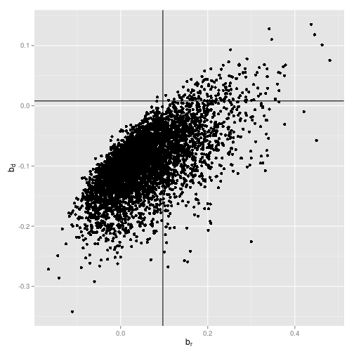
ggplot(reg_coef[1:min(nrMCS, 5000), ], aes(x=Coef_ret, y=Coef_div_growth)) +
geom_point() +
geom_vline(xintercept=0.097) +
geom_hline(yintercept=0.008) +
xlab(expression(b[r])) +
ylab(expression(b[d]))
#Plot maximum 5000 points
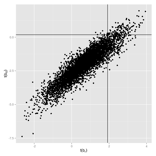
ggplot(reg_coef[1:min(nrMCS, 5000), ], aes(x=tValue_ret, y=tValue_div_growth)) +
geom_point() +
geom_vline(xintercept=1.92) +
geom_hline(yintercept=0.18) +
xlab(expression(t(b[r]))) +
ylab(expression(t(b[d])))
Cochrane's main point in this study is that when you just look at the regression coefficient of the log dividend yield on log returns, you would find quite often coefficents as large as or larger than the $0.097$ in the data, even if the true underlying coefficient is zero. Those are basically all data points right to the vertical line in the plot. The reason we get those significant coefficients and t-values even in a simulated world in which the true underlying coefficient is zero is due to econometrical issues. Concretely, the independent variable, i.e. the dividend yield, is very persistent and the errors are highly correlated. Stambaugh (1999) is a great start if you want to learn more about that.
But Cochrane argues that you shouldn't just look at the regression coefficient on log returns because by definition, either log returns or log dividend growth or both have to be predictable. So if we find positive return coefficients, although return is not predictable, as simulated in his example, then we should also find regression coefficients below $0.008$ for the log dividend yield on log dividend growth. Those are the points below the horizontal line in the plot. However, what we observe in the data is an economically large positive coefficient on log returns and a slightly positive coefficient on log dividend growth and this combination is very unlikely in a world in which log returns are unpredictable.
reg_coef$LRC_ret <- reg_coef$Coef_ret / (1-rho*reg_coef$Coef_dp)
ggplot(reg_coef, aes(x=LRC_ret)) +
  geom_histogram(binwidth=0.05) +
  geom_vline(xintercept = 1.09) +
  xlim(-2, 2)
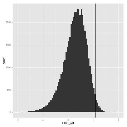
min(reg_coef$LRC_ret)
## [1] -49.15
#Plot maximum 5000 points
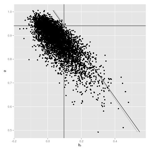
ggplot(reg_coef[1:min(nrMCS, 5000), ], aes(x=Coef_ret, y=Coef_dp)) +
geom_point() +
geom_vline(xintercept=0.097) +
geom_hline(yintercept=phi) +
xlab(expression(b[r])) +
ylab(expression(phi)) +
geom_line(aes(x=1-rho*c(min(Coef_dp),max(Coef_dp)) + 0.008,
y=c(min(Coef_dp),max(Coef_dp))),
linetype="dotted") +
geom_line(aes(x=0.097*(1-rho*c(min(Coef_dp),max(Coef_dp)))/(1-rho*phi),
y=c(min(Coef_dp),max(Coef_dp))))
nrMCS <- 5000 #Otherwise it runs quite long
vec_phi <- c(0.9, 0.941, 0.96, 0.98, 0.99, 1, 1.01)
df <- data.frame(Phi = vec_phi,
                 br  = 0,
                 bd  = 0)
df[, 1] <- vec_phi
i <- 1
for (p in vec_phi) {

  int_reg_coef <- run_MCS(nrMCS = nrMCS, phi=p, rho=rho, nrT = 77, vec_sd = c(0.196, 0.14, 0.153))
  df[i, 2] <- sum(int_reg_coef$Coef_ret > 0.097)/nrMCS*100
  df[i, 3] <- sum(int_reg_coef$Coef_div_growth > 0.008)/nrMCS*100
  i <- i + 1

}
print(xtable(df), type="HTML")
| Phi | br | bd | |
|---|---|---|---|
| 1 | 0.90 | 27.18 | 1.00 |
| 2 | 0.94 | 26.66 | 2.82 |
| 3 | 0.96 | 26.04 | 3.92 |
| 4 | 0.98 | 25.46 | 6.58 |
| 5 | 0.99 | 24.30 | 8.66 |
| 6 | 1.00 | 25.84 | 11.44 |
| 7 | 1.01 | 22.14 | 13.28 |
colMeans(reg_coef)[1:3]
##        Coef_ret Coef_div_growth         Coef_dp
##         0.05708        -0.09323         0.88160
blog comments powered by Disqus